Cell Atlas of Worm

Introduction

This notebook will show you how to work with the C. elegans L2-stage sci-RNA-seq data from Cao et al. (Science, 2017). It aims to cover the following use cases:

Accessing the raw data
Exploring the expression pattern of a gene interest
Finding differentially expressed genes between subsets of cells
Re-clustering subsets of the data using t-SNE

Key advantages of sci-RNA-seq over contemporary alternatives (such as droplet-based single cell RNA-seq):

sublinear cost scaling
reliance on widely available reagents and equipment
ability to concurrently process many samples within a single workflow
compatibility with methanol fixation of cells
cell capture based on DNA content rather than cell size
the flexibility to profile either cells or nuclei

Installation

Required R Packages

dplyr
ggplot2
monocle version 2.3.5

Monocle is a comprehensive package for single cell analysis developed by the Trapnell lab. Monocle version 2.3.5 is the version that was used for the paper. To install Monocle 2.3.5, open a command line and run:

            curl -O http://waterston.gs.washington.edu/sci_RNA_seq_gene_count_data/monocle_2.3.5.tar.gz
            R CMD INSTALL monocle_2.3.5.tar

Later versions of Monocle may produce different results for use case 4 (re-clustering with t-SNE) due to changes in how we preprocess the data before running t-SNE. We will update this vignette when we release the next version of Monocle, 2.6.0, to support the new version. If you wish to learn more about Monocle click the following link to go to the Monocle Website .

Now, go back to your R session and verify that Monocle 2.3.5 installed successfully (look for monocle_2.3.5 in the output of sessionInfo).

            suppressPackageStartupMessages({
              library(monocle)
              library(dplyr)
              library(ggplot2)
            })

            sessionInfo()

Next, we'll download an RData file that has the Cao et al. data and some utility functions to help navigate it.

          download.file(
            "http://waterston.gs.washington.edu/sci_RNA_seq_gene_count_data/Cao_et_al_2017_vignette.RData",
            destfile = "Cao_et_al_2017_vignette.RData")

            load("Cao_et_al_2017_vignette.RData")
            ls()

Important Information

cds is a Monocle CellDataSet object containing the single cell RNA-seq data from the main L2-stage C. elegans experiment described in Cao et al., along with annotations.
cds.neurons is a re-clustered subset of the neuronal cells from cds.
cds.experiment.2 has data from the second C. elegans experiment described in Cao et al.. This includes intestine cells that were missed in the first experiment, but the data overall is lower quality than the first experiment. In the manuscript, we only included the intestine cells from this experiment and excluded the rest.

Do Not Open GitHub Issues for Questions

If you need help or have any questions, submit your posts to the Google Group. If you find a problem with the code in the vignettes or with the data quality, open a GitHub issue.

Use Case 1: Accessing the Raw Data

To this end, we have created a website to facilitate the further annotation of these data by the community (http://atlas.gs.washington.edu). Gene-by-cell matrices and vignettes for how to work with the data are also hosted at this site.

If you aren't familiar with working with single cell RNA-seq data, we highly recommend that you take a look at the examples and utility functions presented in the other sections of this document instead of trying to dive in to the raw data directly.

            exprs(cds)[1:3, 1:3]

3 x 3 sparse Matrix of class "dgCMatrix"

	cele-001-001.CATGACTCAA	cele-001-001.AAGACGGCCA
WBGene00000001	.	.
WBGene00000002	.	.
WBGene00000003	.	.
	cele-001-001.GCCAACGCCA
WBGene00000001	.
WBGene00000002	.
WBGene00000003	.

          fData(cds)[1:3,]

	gene_id	symbol	num_cells_expressed
WBGene00000001	WBGene00000001	aap-1	1016
WBGene00000002	WBGene00000002	aat-1	354
WBGene00000003	WBGene00000003	aat-2	897

The pData function is used to access cell annotations.

annotation	description
`n.umi`	the number of unique molecular identifiers observed to be expressed by a given cell
`Size_Factor`	n.umi divided by the geometric mean of n.umi across all cells
`tsne_1` and `tsne_2`	the coordinates for the cell in the t-SNE dimensionality reduction
`Cluster`	the cluster id assigned by the density peak clustering algorithm
`cell.type` and `tissue`	the cluster id assigned by density peak clustering algorithm applied on the first two t-SNE reduced dimensions

          pData(cds)[1:3,]

	cele-001-001.CATGACTCAA	cele-001-001.AAGACGGCCA	cele-001-001.GCCAACGCCA
cell	cele-001-001.CATGACTCAA	cele-001-001.AAGACGGCCA	cele-001-001.GCCAACGCCA
n.umi	144	790	832
plate	001	001	001
Size_Factor	0.2368328	1.2992911	1.3683674
num_genes_expressed	89	419	338
tsne_1	5.4866377	-3.8619751	-0.5594413
tsne_2	14.67085	-27.63448	41.98569
Cluster	20	6	13
peaks	FALSE	FALSE	FALSE
halo	TRUE	TRUE	TRUE
delta	0.02491657	0.40961274	0.04445184
rho	893.9855	812.2076	240.2908
cell.type	Unclassified neurons	Germline	Intestinal/rectal muscle
tissue	Neurons	Gonad	Intestinal/rectal muscle

neuron.type in pData(cds.neurons) is the annotation used in Figure 4 of Cao et al.

	cele-001-001.CATGACTCAA	cele-001-001.AACTACGGCT	cele-001-001.GAGGCTTATT
cell	cele-001-001.CATGACTCAA	cele-001-001.AACTACGGCT	cele-001-001.GAGGCTTATT
n.umi	144	201	117
plate	001	001	001
Size_Factor	0.2368328	0.3305791	0.1924267
num_genes_expressed	89	129	76
tsne_1	0.9574604	-3.0567593	-18.5689290
tsne_2	0.8288424	-41.4083795	-33.9833909
Cluster	11	8	39
peaks	FALSE	FALSE	FALSE
halo	TRUE	TRUE	TRUE
delta	0.37046400	0.25861943	0.02962754
rho	108.71265	70.88069	37.29414
cell.type	Unclassified neurons	Ciliated sensory neurons	Ciliated sensory neurons
tissue	Neurons	Neurons	Neurons
neuron.type	Cholinergic (11)	ASI/ASJ	AFD

Use Case 2: Expression Pattern of a Gene of Interest

The show.expr.info function returns statistics related to the expression of a given gene in tabular form. The first argument is the gene name. The second argument specifies whether to show statistics at the level of tissues, cell types, or neuron (sub)-types. See the examples below.

the function returns a data frame with five columns:

name	description
`facet`	the tissue / cell type / neuron type
`tpm`	the expression of the given gene in the facet in TPM (transcripts per million)
`prop.cells.expr`	the proportion of cells in the facet that express at least one UMI (unique molecular identifier) for the given gene. Note that cells in different facets can have very different average number of UMIs per cell, so TPM is the better measure of relative expression.
`n.umi`	the number of UMIs (unique molecular identifiers) observed for the given gene in the facet. This is the "sample size" from which the TPM value is computed
`total.n.umi.for.facet`	the total number of UMIs observed across all genes for all cells in the facet

RNA Leakage

Note that low levels of expression of a given gene in cell types you would not expect may be due to leakage of RNA in the fixed cells. For this experiment, based on the expression patterns for a few marker genes, we estimate that the background level of expression you will observe randomly in cells that do not truly express a given gene is ~1-2% of the expression of the highest-expressing cell type.

            show.expr.info("emb-9", "tissue")

facet	tpm	props.cells.expr	n.umi	total.n.umi.for.facet
Body wall muscle	7972.27222	0.96451347	157028	19390434
Gonad	390.16652	0.03757116	3597	11166871
Intestine	597.88569	0.09775967	102	1230975
Neurons	89.83882	0.01406926	187	2203067
Gila	72.96189	0.02148228	39	787560
Pharynx	165.1210	0.01592357	14	85381
Hypodermis	47.05950	0.01821904/th>	158	5821384

              show.expr.info("emb-9", "cell type") %>% head(10)

facet	tpm	prop.cells.expr	n.umi	total.n.umi.for.facet
Distal Tip Cells	16165.1598	0.97520661	3405	202581
Body wall muscle	7972.2722	0.96451347	157028	19390434
Intestinal/rectal muscle	5211.8861	0.84740260	2622	439170
Sex myoblasts	218.2425	0.14776632	75	377288
Pharyngeal neurons	165.1210	0.01592357	14	85381
Other interneurons	137.8986	0.02483070	17	172852
Socket Cells	123.7517	0.02793296	26	184774
Coelomocytes	115.4683	0.02503682	71	544263
Non-seam hypodermis	102.4186	0.02006689	56	1059546
Somatic gonad precursors	102.1766	0.06376812	75	823856

          show.expr.info("R102.2", "neuron type") %>% head(10)

facet	tpm	prop.cells.expr	n.umi	total.n.umi.for.facet
Cluster 21	9807.74014	0.91588785	446	49587
Cluster 16	8266.64832	0.66025641	363	47719
ASK	6720.61429	0.81944444	155	24157
ASI/ASJ	6482.22237	0.74358974	239	40396
ASG	2121.04289	0.39534884	48	26295
ASEL	1670.50501	0.37837838	17	11042
ASER	795.91129	0.28571429	16	15324
AWB/AWC	85.09161	0.02380952	4	23186
Cholinergic (15)	60.56935	0.01538462	1	14463
Pharyngeal (33)	58.35581	0.02857143	2	25101

Source Code of Utility Functions

Note that you can see the source code for any of the utility functions used in this vignette. Just run the function name with no parentheses.

          show.expr.info

            function (gene, expr.info)
            {
                if (class(expr.info) == "character") {
                    expr.info = gsub("[.]", " ", tolower(expr.info))
                    if (expr.info == "tissue")
                        expr.info = tissue.expr.info
                    else if (expr.info == "cell type")
                        expr.info = cell.type.expr.info
                    else if (expr.info == "neuron type")
                        expr.info = neuron.type.expr.info
                }
                gene.id =
                  get.gene.id(gene, fData.df = expr.info$gene.annotations)
                data.frame(facet = names(expr.info$tpm[gene.id, ]),
                tpm = expr.info$tpm[gene.id,],
                prop.cells.expr = expr.info$prop.cells.expr[gene.id,],
                n.umi = expr.info$n.umi[gene.id, ],
                total.n.umi.for.facet = expr.info$total.n.umi.for.facet)
                  %>% arrange(-tpm)
            }

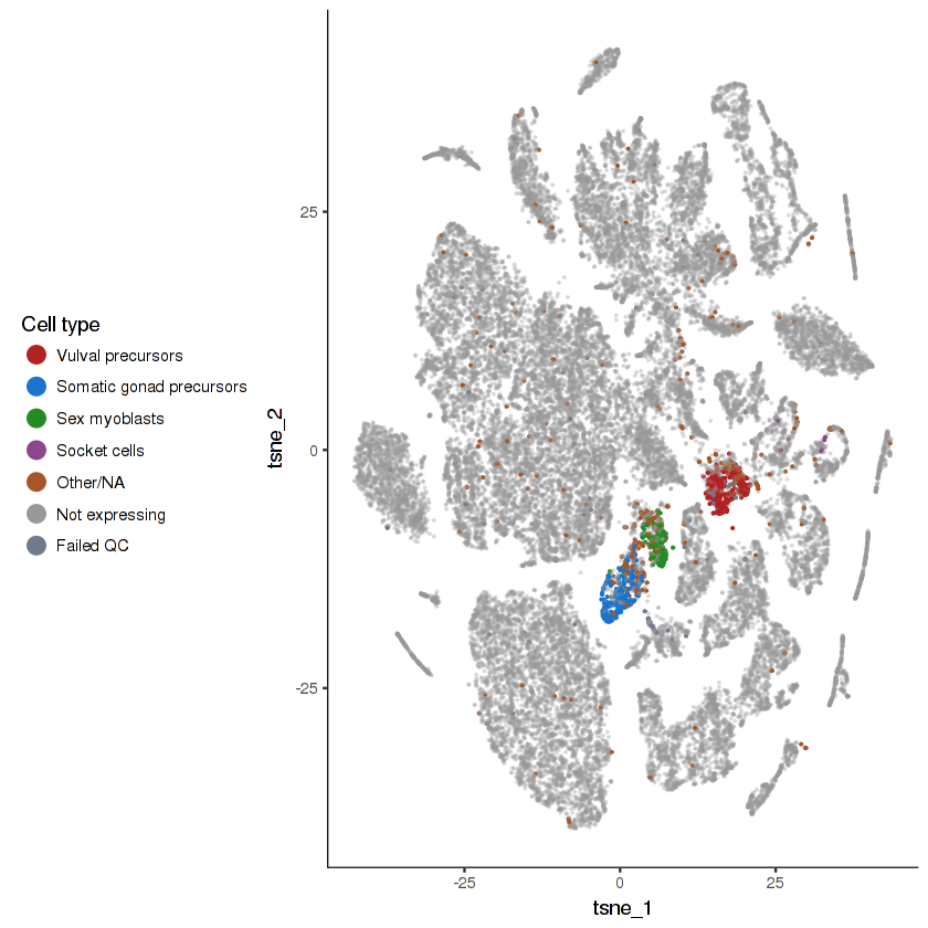
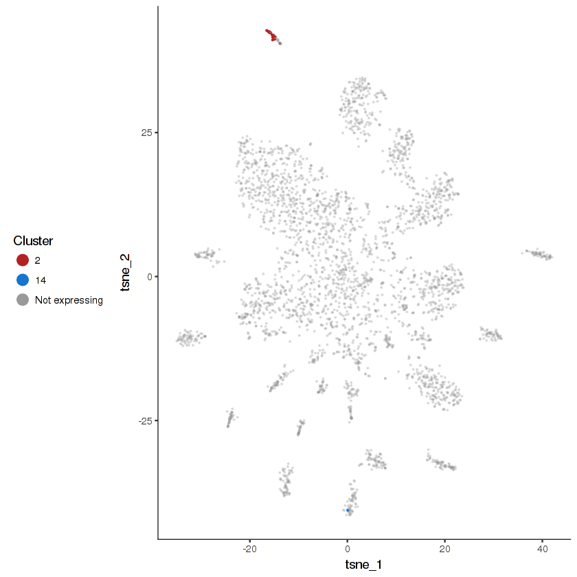
The plot.expr function can be used to highlight cells that express a given gene on the t-SNE map.

Cells that do not express the gene will be colored grey. They are made semi-transparent so as to better highlight the cells that do express the gene.
Cells that express the gene will be colored according to their cell type. The top 4 highest-expressing cell types will be assigned distinct colors. Other cell types will be lumped together.
Cells in the "Failed QC" category are those that express the gene, but are excluded from the analysis due to either having an unusually low UMI count or being a likely doublet.

            plot.expr(cds, "lin-12")

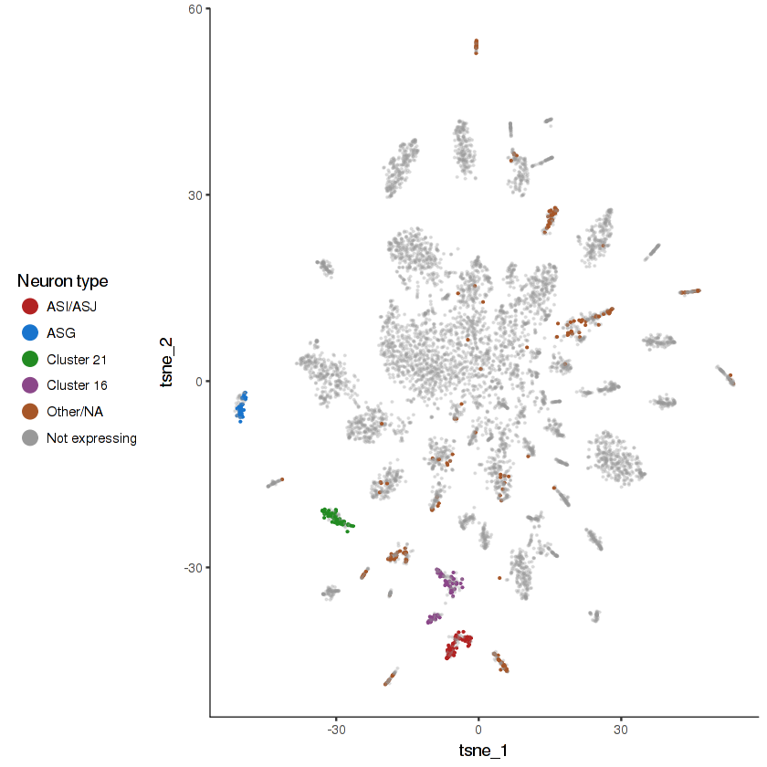
            plot.expr(cds.neurons, "che-3")

Use Case 3: Differential expression between cell subsets

We've defined a function two.set.differential.gene.test that finds and reports statistics on differentially expressed genes (DEG) that distinguish between two defined sets of cells. This is a wrapper that just adds a bit of functionality around Monocle's differentialGeneTest function.

two.set.differential.gene.test takes four arguments:

argument	description
`cds`	a CellDataSet object that includes both sets of cells you wish to compare
`set.1.filter`	a boolean vector of length ncol(cds) indicating which cells should be in Set 1
`set.2.filter`	a boolean vector of length ncol(cds) indicating which cells should be in Set 2
`formal`	if TRUE, p-values and q-values are computed for differential gene expression and genes are ranked by q-value. if FALSE, no formal statistical test is performed and genes are heuristically ranked. formal = F makes the function run much, much faster

Large Memory Use for Differential Expression Tests

If you run two.set.differential.gene.test on large sets of cells (> 1000-ish), it may take a bunch of memory. The utility functions is.tissue, is.cell.type, and is.neuron.type may be used to create the boolean vectors required for the set.1.filter and set.2.filter parameters. Each function takes a CellDataSet and a string and tests for each cell whether its tissue / cell type / neuron type is defined (not NA) and equal to the given value.

          is.tissue

          function (cds, x)
          {
              with(pData(cds), !is.na(tissue) & tissue == x)
          }

            head(is.tissue(cds, "Gonad"))

            > FALSE TRUE FALSE FALSE FALSE TRUE

            sum(is.tissue(cds, "Gonad"))

            > 5628

          sum(is.cell.type(cds, "Distal tip cells"))
          sum(is.neuron.type(cds.neurons, "ASEL"))

          > 129
          > 37

            tissues

            > 'Body wall muscle' 'Pharynx' 'Hypodermis' 'Neurons' 'Gila' 'Gonad' 'Intestine'

            cell.types

            > 'Am/PH sheath cells' 'Body wall muscle' 'Canal associated neurons'
            'Cholinergic neurons' 'Ciliated sensory neurons' 'Coelomocytes' 'Distal tip cells'
            'Dopaminergic neurons' 'Excretory cells' 'flp-1(+) interneurons'
            'GABAergic neurons' 'Germline' 'Intestinal/rectal muscle' 'Intestine'
            'Non-seam hypodermis' 'Other interneurons' 'Oxygen sensory neurons'
            'Pharyngeal epithelia' 'Pharyngeal gland' 'Pharyngeal muscle' 'Pharyngeal neurons'
            'Rectum' 'Seam cells' 'Sex myoblasts' 'Socket cells' 'Somatic gonad precursors'
            'Touch receptor neurons' 'Vulval precursors'

            neuron.types
            'AFD' 'ASEL' 'ASER' 'ASG' 'ASI/ASJ' 'ASK' 'AWA' 'AWB/AWC' 'BAG' 'CAN'
            'Cholinergic (11)' 'Cholinergic (15)' 'Cholinergic (23)' 'Cholinergic (24)'
            'Cholinergic (26)' 'Cholinergic (29)' 'Cholinergic (3)' 'Cholinergic (35)'
            'Cholinergic (36)' 'Cluster 10' 'Cluster 13' 'Cluster 16' 'Cluster 17'
            'Cluster 21' 'Cluster 25' 'Cluster 27' 'Cluster 40' 'Cluster 5' 'Dopaminergic'
            'DVA' 'flp-1(+)' 'GABAergic' 'Pharyngeal (33)' 'Pharyngeal (37)' 'PVC/PVD'
            'RIA' 'RIC' 'SDQ/ALN/PLN' 'Touch receptor' 'URX/AQR/PQR'

          ASEL.vs.ASER.DEG = two.set.differential.gene.test(
            cds.neurons, is.neuron.type(cds.neurons, "ASEL"),
              is.neuron.type(cds.neurons, "ASER"))

two.set.differential.gene.test returns the following statistics:

argument	description
`set.1.umi`	the number of UMI (unique molecular identifiers) observed for the gene in Set 1
`set.2.umi`	the number of UMI (unique molecular identifiers) observed for the gene in Set 2
`set.1.tpm`	gene expression in Set 1 in TPM (transcripts per million)
`set.2.tpm`	set.2.tpm -- gene expression in Set 2 in TPM (transcripts per million)
`higher.expr`	the number of UMI (unique molecular identifiers) observed for the gene in Set 1
`log2.ratio`	the number of UMI (unique molecular identifiers) observed for the gene in Set 2
`precision`	gene expression in Set 1 in TPM (transcripts per million)
`recall`	set.2.tpm -- gene expression in Set 2 in TPM (transcripts per million)
`f.score`	harmonic mean of precision and recall. genes are sorted by this metric

            ASEL.vs.ASER.DEG %>% head()

gene	tank-1	gcy-22	gei-3	gcy-3	gcy-6	T27C4.1
set.1.n.umi	20	0	10	0	66	30
set.1.n.umi	570	129	166	147	0	164
set.1.tpm	1794.188	0.000	1095.928	0.000	6909.705	3210.293
set.2.tpm	36169.778	8862.360	12076.301	9593.506	0.000	11338.218
higher.expr	Set 2	Set 2	Set 2	Set 2	Set 1	Set 2
log2.ratio	4.332578	13.113475	3.460638	13.227842	12.754408	1.819968
precision	0.8536585	1.0000000	0.9090909	1.0000000	1.0000000	0.6808511
recall	1.0000000	0.8000000	0.8571429	0.7428571	0.7297297	0.9142857
f.score	0.9210526	0.8888889	0.8823529	0.8524590	0.8437500	0.7804878

          ASEL.vs.ASER.DEG %>% filter(higher.expr == "Set 1")
            %>% head()

gene	gcy-6	gcy-17	crh-1	gcy-20	gcy-7	unc-44
set.1.n.umi	66	69	58	53	39	88
set.2.n.umi	0	0	12	0	0	45
set.1.n.tpm	6909.705	6553.874	5675.336	5339.037	3709.660	7647.438
set.2.tpm	0.000	0.000	800.504	0.000	0.000	2915.088
higher.expr	Set 1	Set 1	Set 1	Set 1	Set 1	Set 1
log2.ratio	12.754408	12.678132	2.823924	12.382364	11.857071	1.390942
precision	1.0000000	1.0000000	0.8333333	1.0000000	1.0000000	0.6000000
recall	0.7297297	0.6216216	0.6756757	0.5945946	0.5675676	0.8108108
f.score	0.8437500	0.7666667	0.7462687	0.7457627	0.7241379	0.6896552

Running two.set.differential.gene.test with formal = T will compute q-value (the false detection rate at which a gene can be considered to be differentially expressed between the two sets). This is very slow however, so we recommend not using it for exploratory analysis and only using it after you've found something interesting and want to verify that the finding is statistically robust.

          system.time({
          ASEL.vs.ASER.DEG = two.set.differential.gene.test(
              cds.neurons,
              is.neuron.type(cds.neurons, "ASEL"),
              is.neuron.type(cds.neurons, "ASER"),
              formal = T, cores = min(16, detectCores()))
          })

user	system	elapsed
21.241	3.599	152.575

            ASEL.vs.ASER.DEG %>% head()

gene	tank-1	gcy-22	gei-3	gcy-3	gcy-6	T27C4.1
set.1.n.umi	20	0	10	0	66	30
set.2.n.umi	570	129	166	147	0	164
set.1.tpm	1794.188	0.000	1095.928	0.000	6909.705	3210.293
set.2.tpm	36169.778	8862.360	12076.301	9593.506	0.000	11338.218
higher.expr	Set 2	Set 2	Set 2	Set 2	Set 1	Set 2
log2.ratio	4.332578	13.113475	3.460638	13.227842	12.754408	1.819968
precision	0.8536585	1.0000000	0.9090909	1.0000000	1.0000000	0.6808511
recall	1.0000000	0.8000000	0.8571429	0.7428571	0.7297297	0.9142857
f.score	0.9210526	0.8888889	0.8823529	0.8524590	0.8437500	0.7804878

           touch.receptor.neurons.DEG  %>% filter(higher.expr == "Set 1") %>% head()

gene	mec-17	mec-18	mtd-1	mec-7	mec-1	mec-9
set.1.n.umi	2720	796	443	4418	1717	726
set.2.n.umi	118	49	15	743	695	337
set.1.tpm	24033.028	7040.671	4025.528	35936.308	16304.188	7088.606
set.2.tpm	39.202902	17.963804	5.513083	239.162028	328.822706	182.571539
higher.expr	Set 1	Set 1	Set 1	Set 1	Set 1	Set 1
log2.ratio	9.223503	8.536321	9.271622	7.225290	5.627408	5.271088
precision	0.9009288	0.9094828	0.9476440	0.5563771	0.4609610	0.5126263
recall	0.8712575	0.6317365	0.5419162	0.9011976	0.9191617	0.6077844
f.score	0.8858447	0.7455830	0.6895238	0.6880000	0.6140000	0.5561644

tni-3 is a troponin that is expressed in body wall muscle (BWM) in the head, but not in the posterior.
cwn-1 and egl-20 are Wnt ligands that are expressed in posterior BWM, but not anterior BWM.

Using these genes as markers, let's look for differentially expressed genes between anterior and posterior BWM.

          BWM.anterior.vs.posterior.DEG =
            two.set.differential.gene.test(
              cds,
              is.cell.type(cds, "Body wall muscle") &
                expresses.gene(cds, "tni-3"),
              is.cell.type(cds, "Body wall muscle") &
                (expresses.gene(cds, "cwn-1") |
            expresses.gene(cds, "egl-20")))

          BWM.anterior.vs.posterior.DEG$higher.expr = ifelse(
              BWM.anterior.vs.posterior.DEG$higher.expr == "Set 1",
              "Anterior BWM", "Posterior BWM")

gene	set.1.n.umi	set.2.n.umi	set.1.tpm	set.2.tpm	higher.expr	log2.ratio	precision	recall	f.score
tni-13	6981	93	3804.24742	18.57887	Anterior BWM	7.602169	0.9819890	1.0000000	0.9909127
cwn-1	59	3113	13.99762	1311.17230	Posterior BWM	6.449980	0.9821732	0.8968992	0.9376013
T21B6.3	13869	271	5966.03306	60.20010	Anterior BWM	6.607094	0.9553265	0.8867624	0.9197684
glc-4	684	37	310.53057	11.4323046	Anterior BWM	4.642570	0.9506849	0.2767145	0.4286597
tre-3	555	5	214.79033	0.6369876	Anterior BWM	7.035742	0.9852399	0.2129187	0.3501639
F48E3.8	402	1	144.96720	0.1162907	Anterior BWM	7.020870	0.9947917	0.1523126	0.2641770
dpyd-1	289	6	91.93291	0.9050051	Anterior BWM	5.592715	0.9740933	0.1499203	0.2598480
ceh-34	307	2	131.08432	0.2528051	Anterior BWM	6.709189	0.9885057	0.1371611	0.2408964
seb-2	201	5	85.08025	0.6848107	Anterior BWM	5.658166	0.9750000	0.1244019	0.2206506
sfrp-1	335	2	145.18286	0.2754131	Anterior BWM	6.830763	0.9863946	0.1156300	0.2069950
F35C11.5	168	1	67.97453	0.5230727	Anterior BWM	5.479937	0.9923664	0.1036683	0.1877256

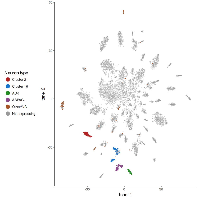
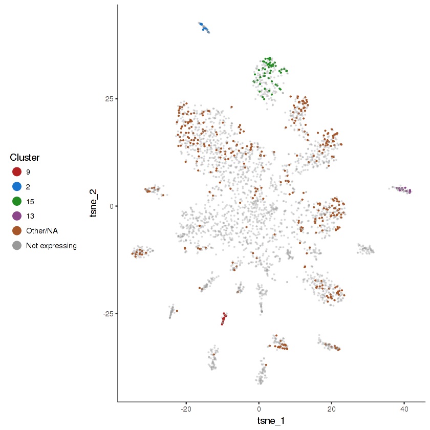
R102.2 is expressed in nine specific pairs of ciliated sensory neurons . We have identified some of these in this dataset, but others remain ambiguous.

            show.expr.info("R102.2", "neuron type") %>% head(8)

facet	tpm	prop.cells.expr	n.umi	total.n.umi.for.facet
Cluster 21	9807.74014	0.91588785	446	49587
Cluster 16	8266.64832	0.66025641	363	47719
ASK	6720.61429	0.81944444	155	24157
ASI/ASJ	6482.22237	0.74358974	239	40396
ASG	2121.04289	0.39534884	48	26295
ASEL	1670.50501	0.37837838	17	11042
ASER	795.91129	0.28571429	16	15324
AWB/AWC	85.09161	0.02380952	4	23186

          plot.expr(cds.neurons, "R102.2")

two.set.differential.gene.test can be used to find DEG between the mystery R102.2(+) clusters and other ciliated sensory neurons. If you can figure out what these clusters correspond to, let us know!

          neuron.cluster.21.vs.other.CSN.DEG =
            two.set.differential.gene.test(
              cds.neurons,
              is.neuron.type(cds.neurons, "Cluster 21"),
              !is.neuron.type(cds.neurons, "Cluster 21") &
              is.cell.type(cds.neurons, "Ciliated sensory neurons"))

          neuron.cluster.21.vs.other.CSN.DEG$higher.expr = ifelse(
            neuron.cluster.21.vs.other.CSN.DEG$higher.expr == "Set 1",
            "Cluster 21", "Other CSN")

            neuron.cluster.21.vs.other.CSN.DEG %>%
              filter(higher.expr == "Cluster 21",
            precision >= 0.8) %>% head(10)

gene	set.1.n.umi	set.2.n.umi	set.1.tpm	set.2.tpm	higher.expr	log2.ratio	precision	recall	f.score
C39D10.2	226	1	5237.910	1.667334	Cluster 21	10.939377	0.9880952	0.7757009	0.8691099
T09B9.3	197	0	3836.121	0.000000	Cluster 21	11.905433	1.0000000	0.6074766	0.7558140
F15A4.5	157	15	3677.812	67.963116	Cluster 21	5.736879	0.8923077	0.5420561	0.6744186
flp-25	100	7	1775.299	44.020086	Cluster 21	5.301349	0.9137931	0.4953271	0.6424242
C18H7.6	118	0	2385.147	0.000000	Cluster 21	11.219863	1.0000000	0.4579439	0.6282051
cdh-3	79	11	1811.618	69.489017	Cluster 21	4.683736	0.8809524	0.3457944	0.4966443
K04D7.6	65	0	1110.520	0.000000	Cluster 21	10.117019	1.0000000	0.2710280	0.4264706
C29F4.3	53	0	1067.368	0.000000	Cluster 21	10.059842	1.0000000	0.2523364	0.4029851
K02E2.1	39	0	1084.714	0.000000	Cluster 21	10.083099	1.0000000	0.2523364	0.4029851
dhs-9	67	15	987.323	53.024505	Cluster 21	4.191836	0.8484848	0.2616822	0.4000000

          neuron.cluster.16.vs.other.CSN.DEG =
            two.set.differential.gene.test(
              cds.neurons,
              is.neuron.type(cds.neurons, "Cluster 16"),
              !is.neuron.type(cds.neurons, "Cluster 16") &
                  is.cell.type(cds.neurons,
                "Ciliated sensory neurons"))

          neuron.cluster.16.vs.other.CSN.DEG$higher.expr = ifelse(
            neuron.cluster.16.vs.other.CSN.DEG$higher.expr == "Set 1",
            "Cluster 16", "Other CSN")

            neuron.cluster.16.vs.other.CSN.DEG %>%
                filter(higher.expr == "Cluster 16") %>% head(10)

gene	set.1.n.umi	set.2.n.umi	set.1.tpm	set.2.tpm	higher.expr	log2.ratio	precision	recall	f.score
F27C1.11	223	367	5302.959	1576.21303	Cluster 16	1.7494202	0.3537118	0.5192308	0.4207792
W05F2.7	137	309	3007.794	1054.38784	Cluster 16	1.5109326	0.3564356	0.4615385	0.4022346
M04B2.6	117	4	2144.256	14.78412	Cluster 16	7.0858594	0.9285714	0.2500000	0.3939394
ocr-2	100	81	2408.536	294.50719	Cluster 16	3.0268916	0.5465116	0.3012821	0.3884298
osm-10	66	32	1209.716	124.87432	Cluster 16	3.2646129	0.7222222	0.2500000	0.3714286
R102.2	363	926	8266.648	3753.48748	Cluster 16	1.1386865	0.2524510	0.6602564	0.3652482
T01D3.1	87	122	1849.955	382.64946	Cluster 16	2.2696298	0.4112903	0.3269231	0.3642857
ida-1	337	1211	7843.130	5636.27821	Cluster 16	0.4764307	0.2234848	0.7564103	0.3450292
lap-2	132	55	2344.214	231.93208	Cluster 16	3.3311228	0.5263158	0.2564103	0.3448276
rps-11	83	230	2013.967	1036.83972	Cluster 16	0.9564565	0.2863636	0.4038462	0.3351064

Use Case 4: Re-clustering cell subsets using t-SNE

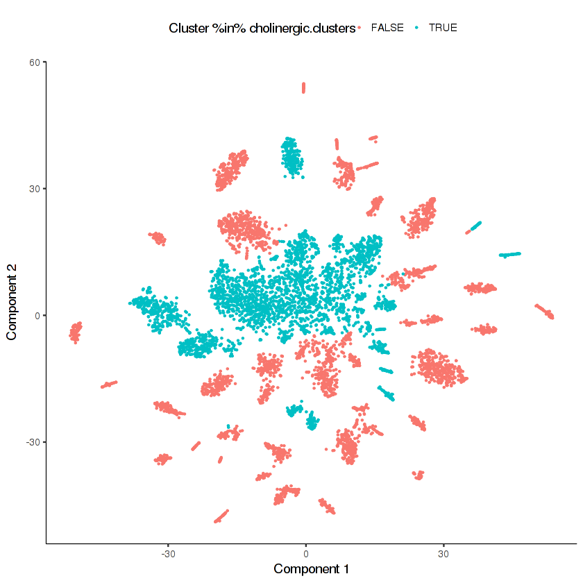
In the Cao et al. paper, we found that several of the neuron t-SNE clusters expressed markers of cholinergic neurons such as unc-17, cho-1, and cha-1. Let's perform a sub-clustering of these cholinergic neurons to see if we can get better separation. First, we'll identify which clusters are enriched for cells that express cholinergic markers.

          pData(cds.neurons)$any.cholinergic.marker =
              (expresses.gene(cds.neurons, "unc-17") +
               expresses.gene(cds.neurons, "cho-1") +
               expresses.gene(cds.neurons, "cha-1")) > 0

          pData(cds.neurons) %>%
              group_by(Cluster) %>%
              summarize(
                  n.total = n(), n.cholinergic =
                    sum(any.cholinergic.marker),
                  prop.cholinergic = n.cholinergic / n.total) %>%
              inner_join(
                  unique(pData(cds.neurons)[, c("Cluster",
                      "neuron.type")]),
                  by = "Cluster") %>%
              arrange(-prop.cholinergic) %>%
              head(15)

Cluster	n.total	n.cholinergic	prop.cholinergic	neuron.type
29	305	155	0.5081967	Cholinergic (29)
23	45	19	0.4222222	Cholinergic (23)
3	385	131	0.3402597	Cholinergic (3)
26	261	81	0.3103448	Cholinergic (26)
35	58	16	0.2758621	Cholinergic (35)
36	128	35	0.2734375	Cholinergic (36)
15	65	16	0.2461538	Cholinergic (15)
12	68	14	0.2058824	DVA
24	188	38	0.2021277	Cholinergic (24)
8	117	23	0.1965812	ASI/ASJ
11	1998	387	0.1936937	Cholinergic (11)
6	160	21	0.1312500	SDQ/ALN/PLN
25	363	43	0.1184573	Cluster 25
41	211	24	0.1137441	Doublets
16	156	17	0.1089744	Cluster 16

          cholinergic.clusters = c(29, 23, 3, 26, 35, 36, 15, 24, 11)
          plot_cell_clusters(cds.neurons, color =
            "Cluster %in% cholinergic.clusters",
            cell_size = 0.2)

          cds.cholinergic =
              cds.neurons[, pData(cds.neurons)$Cluster %in%
                  cholinergic.clusters]
          cat(ncol(cds.cholinergic), "cells in the cds subset", "\n")

          cds.cholinergic = estimateSizeFactors(cds.cholinergic)
          cds.cholinergic = estimateDispersions(cds.cholinergic)
              # above line would take a lot of memory for larger cell sets
          cds.cholinergic = detectGenes(cds.cholinergic, 0.1)

          > 3433 cells in the cds subset

The next step is to run a new t-SNE dimensionality reduction on this subset of cells.

          system.time({
          cds.cholinergic = reduceDimension(
              cds.cholinergic, max_components = 2, norm_method = "log",
              num_dim = 20, reduction_method = 'tSNE', verbose = T)
          })

          pData(cds.cholinergic)$tsne_1 = reducedDimA(cds.cholinergic)[1,]
          pData(cds.cholinergic)$tsne_2 = reducedDimA(cds.cholinergic)[2,]

user	system	elapsed
164.398	2.898	168.483

20 principal components looks like it's enough for this data. If you don't see an elbow in the scree plot, that means you've used too few principal components.

            plot_pc_variance_explained(cds.cholinergic)

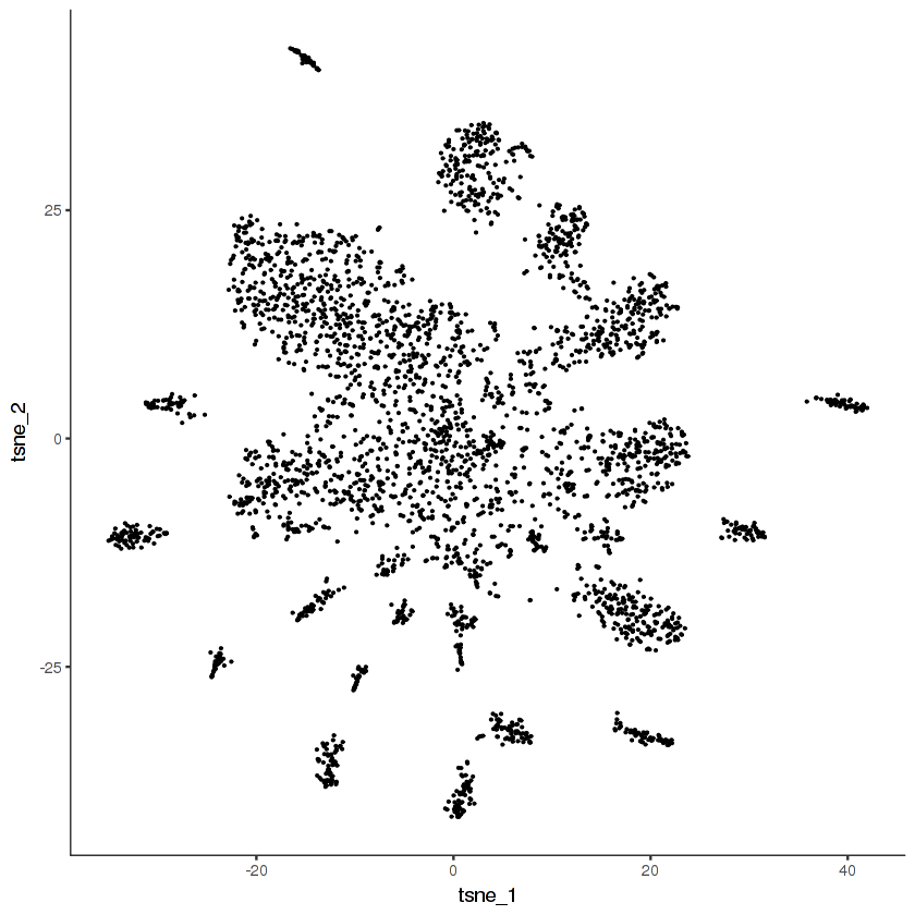
          ggplot(pData(cds.cholinergic), aes(x = tsne_1, y = tsne_2)) +
              geom_point(size = 0.1) +
              monocle:::monocle_theme_opts()

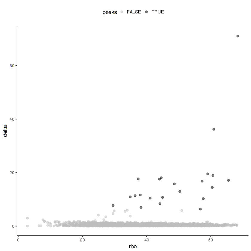
Now we'll cluster the cells in the t-SNE space using density peak clustering. In density peak clustering, rho measures to the local density of cells and delta measures the minimum distance to a region of higher local density. Go to this site for more details. You want to set thresholds on rho and delta that enclose the outlier points in the scatter plot. In my experience, it's usually better to over-cluster than to under-cluster.

            cds.cholinergic = clusterCells_Density_Peak(cds.cholinergic)

            > Distance cutoff calculated to 2.694535

            plot_rho_delta(cds.cholinergic,
              rho_threshold = 10,
              delta_threshold = 6)

          cds.cholinergic = clusterCells_Density_Peak(cds.cholinergic,
              rho_threshold = 10, delta_threshold = 6, skip_rho_sigma = T)
          plot_cell_clusters(cds.cholinergic, cell_size = 0.2)

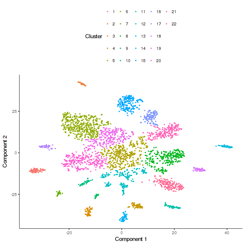
Looks like there are many distinct clusters. Recall that we input only 9 clusters from the cds.neurons t-SNE into this re-clustering. The re-clustering appears to have revealed new potential distinct cell types.

Now would be a good time to save your progress.

            save.image("my_analysis_Cao_et_al_data.RData")

Let's find marker genes for each cluster.

            cholinergic.clusters =
                sort(as.integer(unique(pData(cds.cholinergic)$Cluster)))
            cholinergic.clusters

          > 1 2 3 4 5 6 7 8 9 10 11 12 13 14 15 16 17 18 19 20 21 22

          DEG.results = lapply(cholinergic.clusters,
              function(this.cluster) {
            message("Finding markers for cluster ", this.cluster)
              cbind(
                  two.set.differential.gene.test(
                      cds.cholinergic,
                      pData(cds.cholinergic)$Cluster == this.cluster,
                      pData(cds.cholinergic)$Cluster != this.cluster),
                  data.frame(cluster = this.cluster))
          })

          cholinergic.cluster.markers =
              do.call(rbind, DEG.results) %>%
                  filter(higher.expr == "Set 1") %>%
            select(
                cluster, gene,
                cluster.n.umi = set.1.n.umi,
                other.n.umi = set.2.n.umi,
                cluster.tpm = set.1.tpm,
                other.tpm = set.2.tpm,
                log2.ratio, precision, recall, f.score) %>%
            arrange(-f.score)

            cholinergic.cluster.markers %>%
                filter(precision >= 0.5) %>% head(10)

Cluster	gene	cluster.n.umi	cluster.n.omi	cluster.tpm	other.tpm	log2.ratio	precision	recall	f.score
7	B0432.14	194	11	10886.411	5.8332893	10.637661	0.9047619	0.9500000	0.9268293
13	nlp-42	299	15	22725.799	17.1886827	10.287074	0.8833333	0.9137931	0.8983051
13	nlp-42	299	15	22725.799	17.1886827	10.287074	0.8833333	0.9137931	0.8983051
21	flp-12	1379	297	17963.487	366.8397815	5.609846	0.7282609	0.8777293	0.7960396
13	T04C12.3	173	25	12067.242	22.8874212	8.980629	0.7407407	0.6896552	0.7142857
22	lgc-39	289	93	5300.848	120.7416859	5.444328	0.6346154	0.6839378	0.6583541
1	sem-2	128	63	6240.354	52.4115889	6.868331	0.6615385	0.6056338	0.6323529
2	vglu-2	30	1	2356.216	0.6977763	10.438609	0.9523810	0.4444444	0.6060606
15	Y48C3A.5	339	145	6989.459	148.0684921	5.551134	0.5747664	0.6243655	0.5985401
10	glb-17	81	19	4790.632	16.9955396	8.056433	0.7352941	0.5000000	0.5952381
9	nlp-5	34	24	3552.050	21.1320088	7.326374	0.5500000	0.6470588	0.5945946

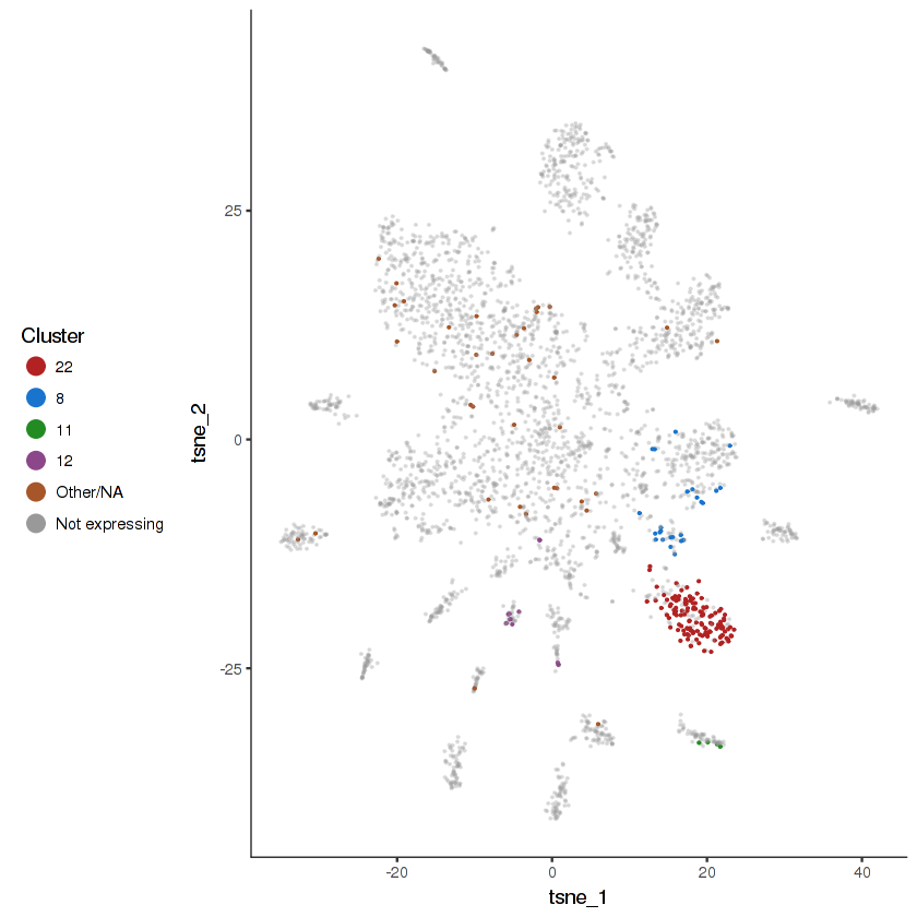
In the previous examples for using plot.expr, the function used pre-computed expression tables for cds and cds.neurons to show which cell types / neuron types were expressing a given gene. The following code will set up plot.expr so it can show which density peak clusters from this re-clustering analysis express a given gene. You can also use show.expr.info with your own clustering.

          cholinergic.expr.info = get.expr.info.by.facet(cds.cholinergic,
            "Cluster")

          plot.expr(cds.cholinergic, "lgc-39", expr.info = cholinergic.expr.info)

          show.expr.info("lgc-39", cholinergic.expr.info) %>% head(10)

facet	tpm	prop.cells.expr	n.umi	total.n.umi.for.facet
21	4677.68319	0.618644068	305	63153
18	244.90291	0.060606061	4	14652
19	232.84907	0.052884615	14	50800
8	217.45530	0.038461538	18	80071
4	155.65487	0.027100271	24	174660
22	129.10174	0.024615385	10	117663
1	79.17593	0.028169014	2	19954
6	60.42661	0.014925373	1	17215
9	56.34438	0.029411765	1	12093
10	30.47108	0.008196721	1	26202

          plot.expr(cds.cholinergic, "vglu-2", expr.info = cholinergic.expr.info)

            show.expr.info("vglu-2", cholinergic.expr.info) %>% head(10)

facet	tpm	prop.cells.expr	n.umi	total.n.umi.for.facet
2	2356.21566	0.44444444	30	11540
14	37.52486	0.01587302	1	23493
1	0.00000	0.00000000	0	19954
3	0.00000	0.00000000	0	19911
4	0.00000	0.00000000	0	174660
5	0.00000	0.00000000	0	51233
6	0.00000	0.00000000	0	17215
7	0.00000	0.00000000	0	17691
8	0.00000	0.00000000	0	80071
9	0.00000	0.00000000	0	12093

              plot.expr(cds.cholinergic, "unc-17", expr.info = cholinergic.expr.info)

          show.expr.info("unc-17", cholinergic.expr.info) %>% head(10)

facet	tpm	prop.cells.expr	n.umi	total.n.umi.for.facet
9	3200.3642	0.3823529	44	12093
2	2944.3520	0.2888889	27	11540
13	2128.1049	0.2500000	29	13140
5	2087.7739	0.2731959	119	51233
15	1992.1189	0.2941176	62	31426
6	1721.6386	0.2686567	34	17215
8	1527.0847	0.1826923	126	80071
4	1344.6852	0.1585366	235	174660
12	1114.1395	0.1718213	123	97104
16	886.1635	0.1923077	16	19103